.png)
This is a highly condensed version of Demystifying Randomness in AI, focusing on position.
Key Takeaways:
1. Position is the rank of an entity within a list of entities, averaged over a sample of AI responses.
2. Measuring position is straightforward. A sample of 10 responses is enough for a quick estimate.
3. For cases that require greater precision, we can use statistical tools to assess the accuracy of position estimates and use sequential sampling to efficiently determine the right number of responses, based on the desired precision and our risk tolerance.
Position Is an Entity’s Rank in a List of Entities
AI often responds differently to the same prompt. However, it is not incoherent. AI randomly samples responses from a probability distribution. This means prompt tracking metrics are measurable using a sample of responses.
When AI responses include a list of entities, we can measure an entity’s position in that list.
For example, in these responses to the prompt “What are the best flavors of ice cream?”,
“Cookies & Cream” appears at positions 5, 4, and 5, and “Coffee” appears at position 9 in the third response, and does not appear in the other responses.
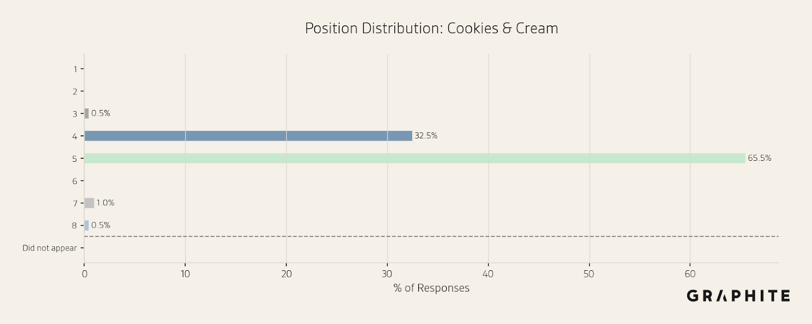
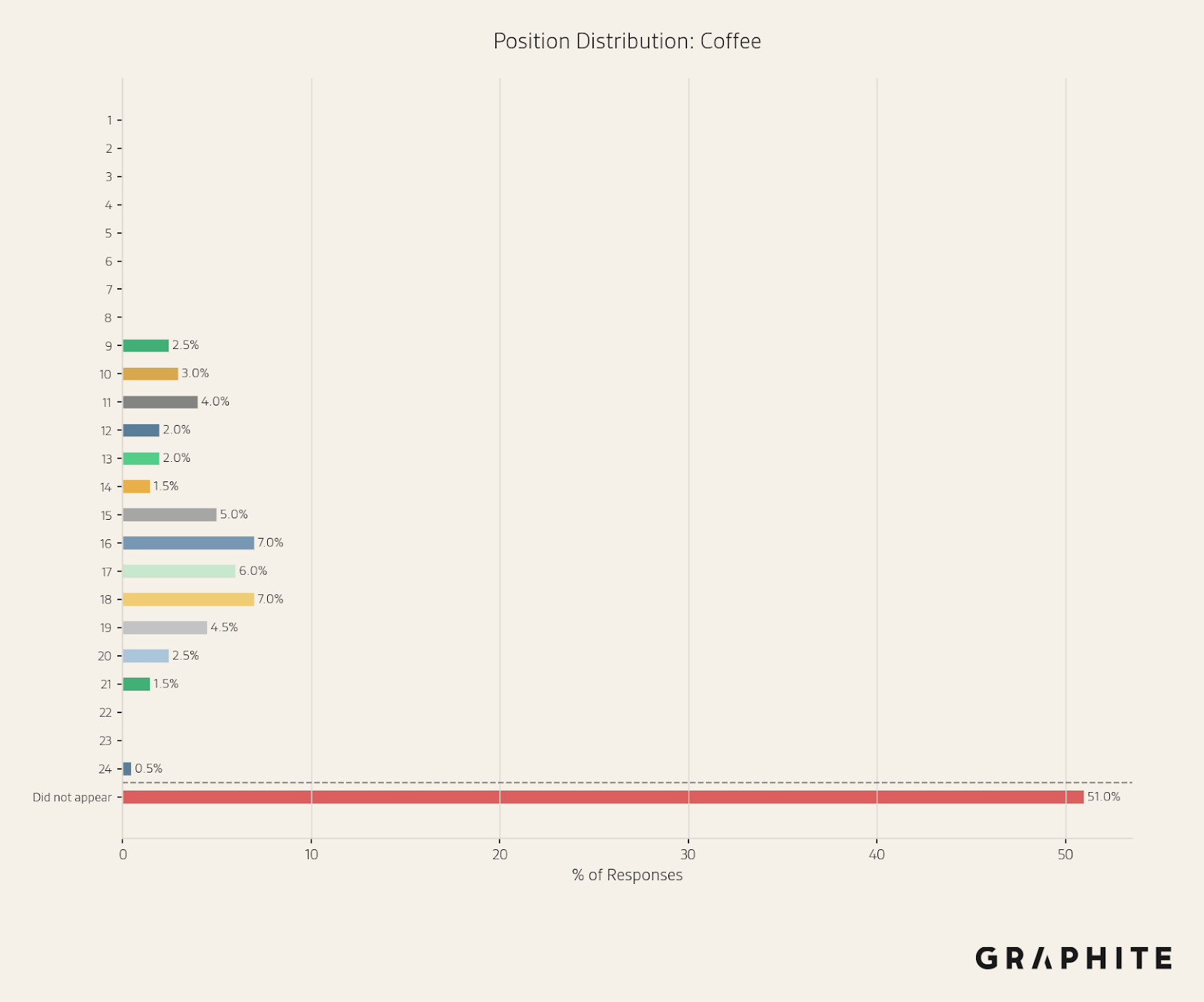
Use Position Histograms to Visualize the Position Distribution
A good way to visualize position over a sample of responses is using a position histogram. It tells us how often an entity appears at a particular position, and how often the entity is not mentioned in the response, which is the complement of its visibility (the percentage of responses that mention an entity).
Cookies & Cream has a relatively stable position distribution.
In contrast, Coffee only appears 49% of the time, and appears at a range of different positions.
Use Average Position to Summarize the Position Distribution
How do we aggregate this into a single value? We take the average position over all the responses where an entity appears. We could instead assign a fake position, like the maximum position in the list plus one, when an entity does not appear, but this makes the position more difficult to interpret.
In the histograms above, the average position for “Cookies & Cream” is 4.7, and the average position for “Coffee” is 15.5.
To help summarize the variability, it is also useful to view the standard deviation of the position across the sample. The standard deviation of position is 0.58 for “Cookies & Cream” and 3.41 for “Coffee”.
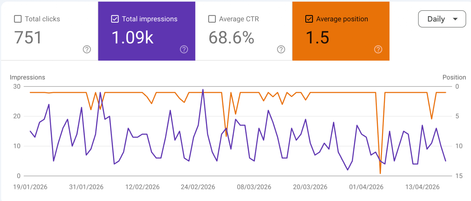
Position Works the Same Way as in Google Search Console (GSC)
Note that despite many claims that AI is very different from traditional search, our definition of position is similar to how position is reported in GSC. A search result can appear in different positions at different times and for different users. GSC provides the average position when the URL appears, as shown in the screenshot below.
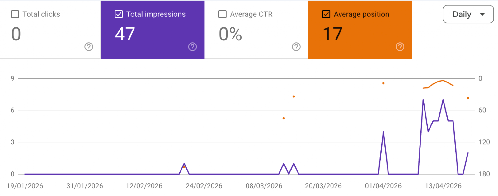
When the URL appears occasionally, the average position ignores cases where the URL does not rank, as shown in the screenshot below.
Focus on Visibility First, Then Position
Visibility and position are complementary. Visibility tells us how often an entity appears, and position provides the average rank when it appears. It does not make sense to focus on position when visibility is low. The first priority is to appear frequently, and the second priority is to appear at the top of the response, as the first recommended item.
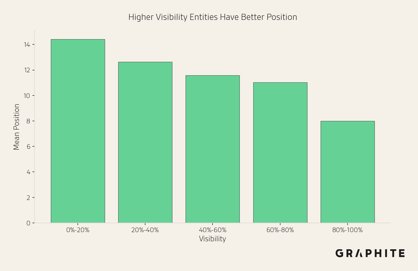
Higher Visibility Implies Better Position
Visibility and position are correlated. Higher visibility generally implies better position.
Top Positions Are More Stable
The top of the list is generally more stable than the bottom.
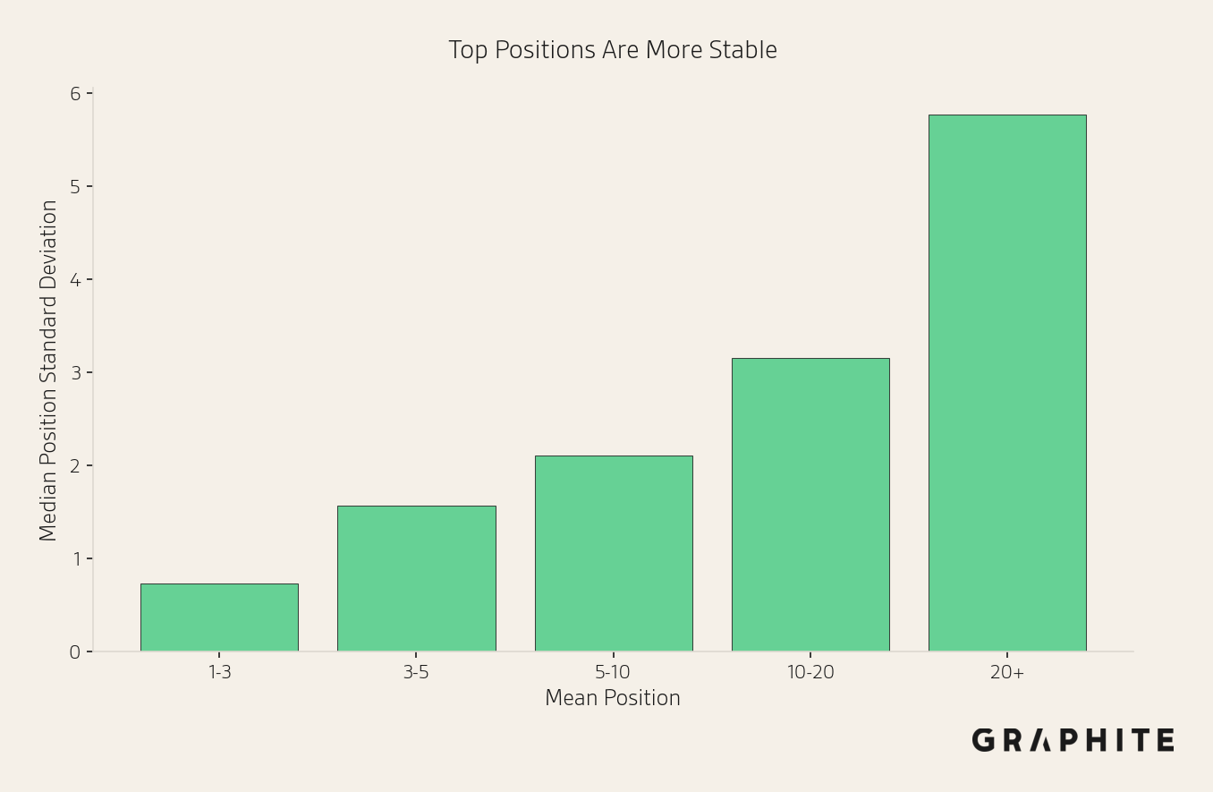
Although position can be highly variable, these two facts combine to make position easier to estimate than we might expect: high-visibility entities, the ones we care about position for, have better and more stable position.
Tracking Position Is Straightforward
We can compute empirical estimation errors to develop rules of thumb for coarse tracking and leverage statistical tools when more precision is needed.
Note that because position is defined only when an entity occurs, the effective sample size for measuring the average position depends on the entity's visibility. Tracking the position of low-visibility entities yields a low effective sample size and unstable estimates, which is another reason to avoid position until visibility is high.
Because we only compute position for entities that appear, entities that do not appear in a sample will not get a position estimate. This means we may underestimate error with very small sample sizes. But by 10 responses, if an entity does not appear, the upper bound of its 95% visibility confidence interval is 27.8%. In this case, we should focus on increasing visibility before considering position.
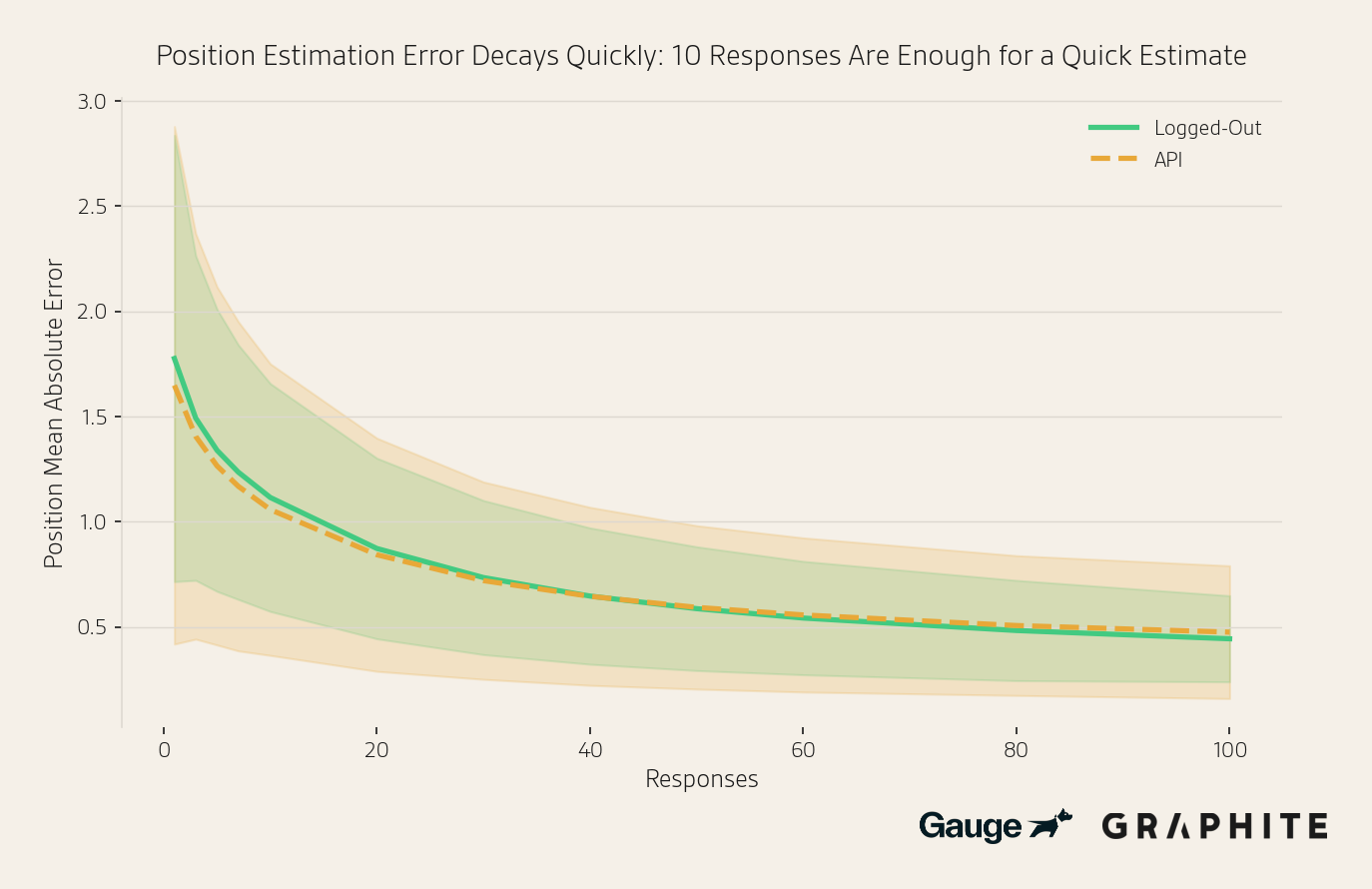
Position Estimation Error Decreases Rapidly with the Number of Responses
We conduct an experiment to measure the mean absolute error in position estimates as a function of the number of responses. For example, if the estimated position is 4.2 and the true position is 5.5, the absolute error is 1.3. The mean absolute error for a prompt is the average absolute error across all entities that appear in the sample. We measure error for entities with visibility of at least 10% in the full set of responses, and we discard entities that do not appear in the sub-sample.
The dataset consists of 200 entity comparison question prompts from three sources: prompts tracked in Graphite’s prompt tracking tool, prompts generated from editorial search keywords, and manually written prompts on topics of general interest, like “What are the best science fiction books right now?” We obtain 400 responses for each prompt from the gpt-5.2-chat-latest model via the OpenAI API and extract entities that are answers to the question. We provide the full dataset of all responses and the entities.
By 10 responses, the position estimation error is just above one position, at 1.06 (out of 23.4 qualifying entities, on average), despite the smaller effective sample size.
In the full paper, we show similar results when:
- Using OpenAI’s API + web search tool
- Using Gemini 3 Flash via API
- Using scraped responses from Gemini
Below, we show the percentage of prompts with a mean absolute error <= 2 or <= 1 position after different numbers of responses using the OpenAI API data. With 10 responses, 90.6% of prompts have a mean absolute error <= 2 positions.
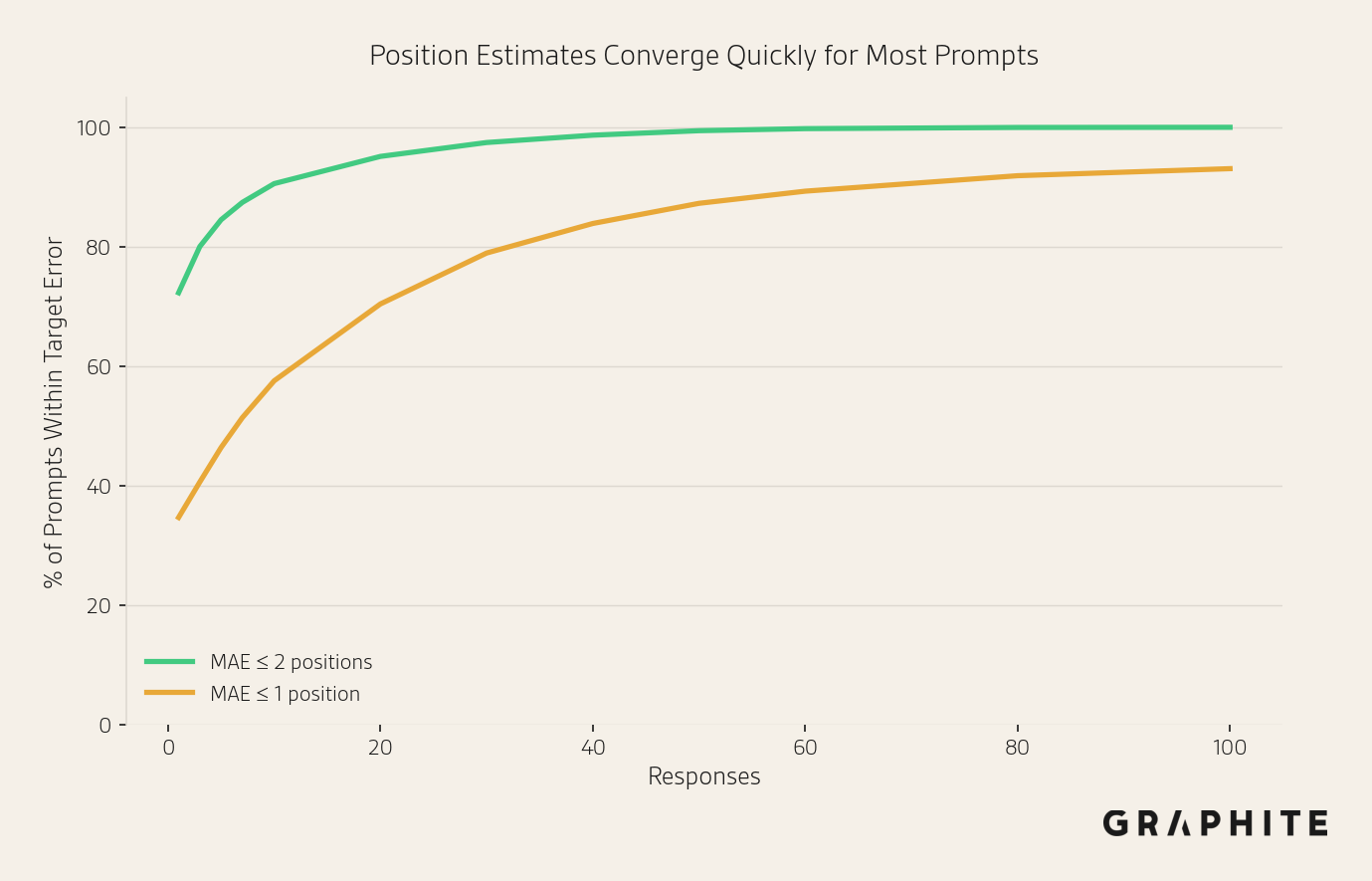
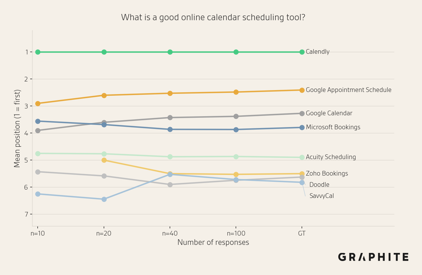
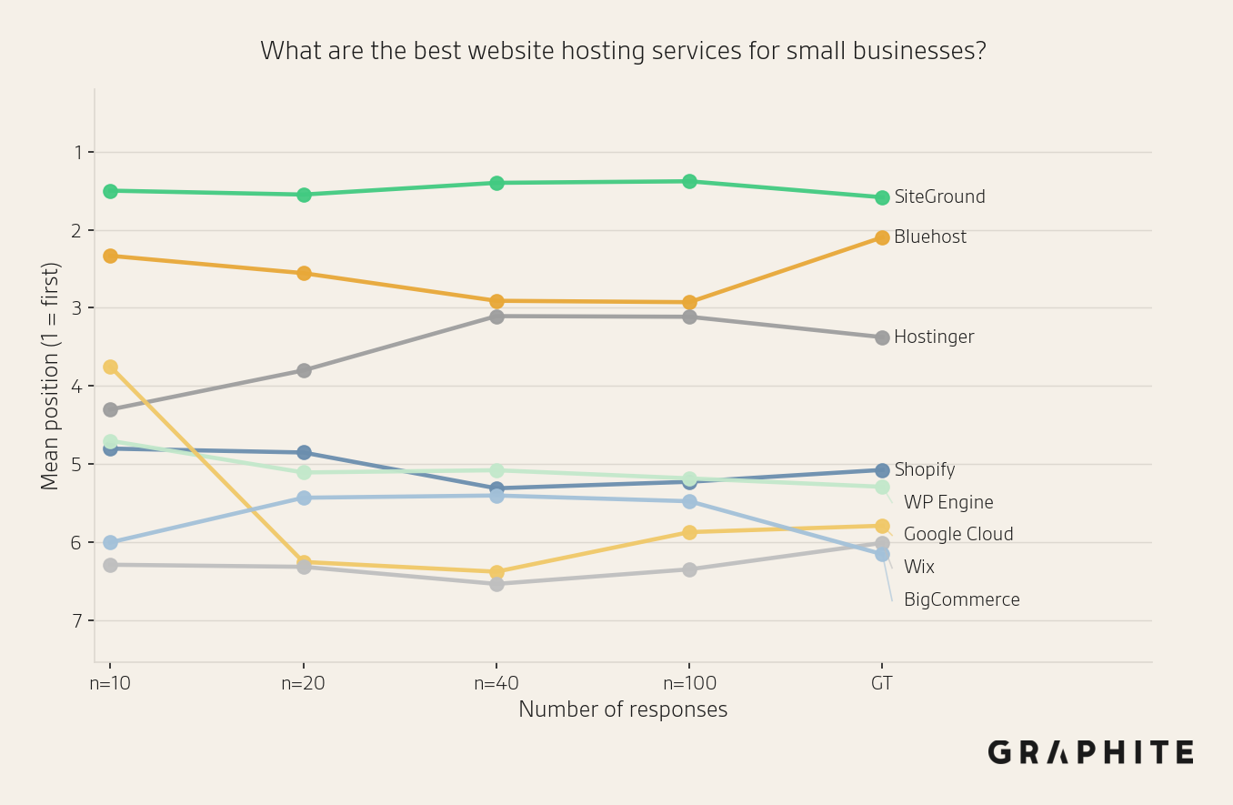
Many of the prompts that do not achieve MAE <= 1 position after 100 samples are “What are the best things to do in CITY?” questions, which have less stable orderings. In contrast, prompts like “What is a good online calendar scheduling tool?” achieve very low MAE (0.27) at 10 responses.
Here are examples of two prompts and their position estimates with different sample sizes. The first stabilizes more quickly than the second.
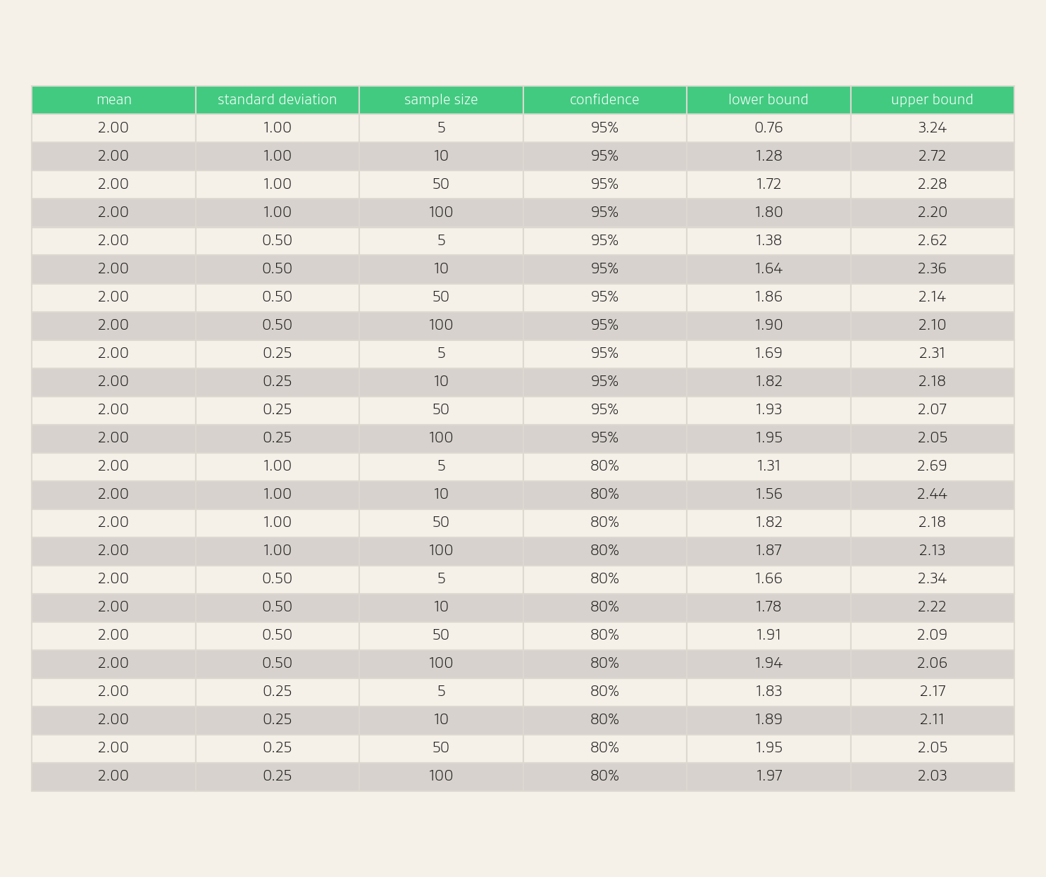
Use Confidence Intervals When You Need More Precision
Confidence intervals are statistical margins of error for estimates. We can compute a confidence interval for the average position using the t-distribution, which accounts for uncertainty in both the sample mean and the sample standard deviation (formula in the full paper Appendix). For this calculation, we need to compute the standard deviation of observed positions. We can see some example confidence intervals in the table below.
Use Sequential Sampling to Decide How Many Responses a Prompt Needs
We can use sequential sampling to decide when an estimate is “good enough”, so that different prompts get different numbers of responses, rather than the common strategy of using a fixed number of responses per prompt, such as 100.
For position, we use a t-distribution-based confidence interval for the mean.
If we want a 95% confidence interval of width less than 2.0 for an entity's mean position, we can iteratively add 10 responses and stop when the width falls below the target. For example, for an entity with an observed position standard deviation of 3.0:
- n=10 => width: 4.29
- n=20 => width: 2.81
- n=30 => width: 2.24
- n=40 => width: 1.92 STOP
The savings provided by stopping early depend on the standard deviation of the entity's position. Entities with stable position (low standard deviation) converge much faster than entities with highly variable position. For example, to get a 95% confidence interval of width 2.0, an entity with standard deviation 0.97 (the 10th percentile in our dataset) needs only 7 responses, whereas an entity with standard deviation 5.87 (the 90th percentile) requires 135 responses, a 95% reduction in samples by stopping early.
In our dataset, 37% of entities with visibility ≥ 10% have position standard deviation below 2.0, and only 16% have a standard deviation above 5.0. On average, achieving a 95% confidence interval of width 2.0 would require 55 responses per entity, a reduction of 59% relative to the worst-case 135. For a confidence interval of width 3.0, the reduction is 58%, from 62 responses to 26.
We could also stop when the average or max width of the confidence interval across all entities reaches a target error width.
For example, for entities with visibility ≥ 10%, suppose we want the average 95% confidence interval width on each prompt to be less than 2.0. Capping sampling at 200 responses per prompt, fixed sampling uses 200 responses on every prompt and meets the target on 88% of prompts. Sequential sampling achieves the same meet-target rate with an average of 85.1 responses per prompt, a 57% reduction.
Position Is Probabilistic but Measurable
Like visibility, position is probabilistic, but measurable using a sample of responses. The full paper Demystifying Randomness in AI covers this (and many other topics) in much more depth.